

The Schwab US Dividend Equity fund launched at the end of 2011 in the relatively early days of a decade-plus bull market in US equities. And yet, through the end of December 2022, it has outperformed the all-cap CRSP US Total Market Index by an annualized 114 basis points on a total return basis. Since inception, the fund boasts a Sharpe Ratio close to 1.0 (0.94), and a Relative Sharpe Ratio 1 19% superior to the broad market factor2, aided considerably by the fund’s lower volatility and just 0.9 exposure to Market Beta.
As summarized in the Factor Tombstone above and reflected in our article covering top-ranked funds on factor capture and valuation, SCHD earns a 100% Relative Factor Capture score, meaning it ranks above the 95% percentile of all funds in our analysis 3 on the basis of Implied Relative Sharpe 4. SCHD realizes meaningful exposure to Value and exceptional exposure to the Profitability and Investment factors.
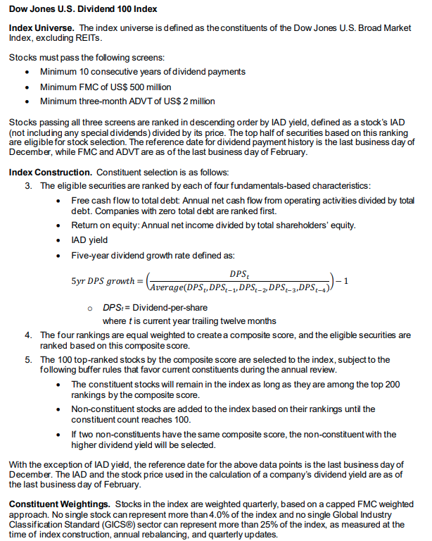
Figure 1 — excerpted from the Dow Jones index literature — transparently outlines the SCHD fund constitution criteria and methodology. As long-only smart beta funds rarely align their constitution criteria explicitly with any given academic factor model 5, we include regressions on the CAPM, FF6, AQR and q5 models for comparison. Table 2 summarizes regression results.
Comparing Schwab US Equity ETF Factor Regressions
Following Table 2 from the top, plain vanilla CAPM establishes the baseline and leaves 300 bps of unexplained alpha with 89% probability of significance (t-stat of 1.6). AQR fits best among the 3 alternative risk premia models, leaving just 22bps of residual alpha (t-stat insignificant). AQR’s Quality Minus Junk (QMJ) factor ostensibly subsumes FF6 CMA and RMW in combination 6 and also sports highly significant exposure to HML. Interestingly, the most statistically-significant individual factor next to AQR HML is the q5 Investment factor (I/A), which is defined as the annual change in total assets; the q5 ROE factor doesn’t register with significance, which is somewhat surprising given its 0.65 correlation with RMW and 0.68 correlation with QMJ. 7
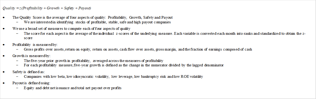
A Logical Mapping of SCHD Criteria to the definition of QMJ
Table 1 maps the DJ 100 criteria detailed in Figure 1 to those of the AQR QMJ factor detailed in Figure 2. QMJ does use z-scoring prior to rank rank weighting, which ought to improve the statistical reliability of the composite. The mapping suggested here could be quantified by constituting and backtesting the DJ 100 Criteria as a factor in its own right (including a short leg composed of equities ranking in the lowest equivalent deciles on these same criteria), and then regressing and comparing with both QMJ and the FF6 CMA and RMW FF6 factors. Qualitatively, the mapping appears straightforward and intuitive.
| DJ 100 Criteria | QMJ Mapping | Reasoning |
|---|---|---|
| Free Cash Flow to Total Debt | Profitability – Cash flow over assets | Equivalent definitions assuming debt as % assets stable across equities |
| ROE | ROE | Identical definition |
| Yield | Total net payout over profits | Yield is a subcomponent of net payout |
| 5Y dividend growth rate | 5Y growth in profitability | Growth in profitability drives dividend growth, all else equal (primary driver of dividend growth likely revenue growth, notwithstanding) |
Factor Contribution Breakdown
Rolling regressions can be used to assess factor stability over time, with factor exposure ideally varying relatively little 8. On a rolling 36-month basis, SCHD factor exposure is very stable through the COVID drawdown of 1H-2022. Factor capture looks considerably different from April 2020 forward, and so we include both sets of summary data here for discussion. The key commonality: CMA and RMW contribution are persistently high and dominant. The Adjusted R^2 (regression goodness of fit) is also notably higher at 0.95 versus just 0.91 when extending the regression through December of 2022.
Figure 3 summarizes the regression coefficients, t-values, and resulting factor contributions when using FF6 regression statistics derived from fund performance through April of 2020 and applied to factor return data from inception through December of 2022. t-statistic and regression coefficient details can be discovered by floating over the graph bar elements. Of note is the significant but comparatively small negative contribution from SMB, the two meaningful 120 bps contributions from CMA and RMA, the statistically-significant contribution from UMD, and the rational negative alpha 9. In sum, the Relative Sharpe of this fund is 1.68, and is our best predictor of what we might expect on an ex-ante basis, assuming that factors deliver their historical mean return premia.
Figure 4 shows how realized factor performance has diverged from the historical mean in the period through April of 2020. HML was negative over the period 10, SMB has a negative correlation coefficient but a positive contribution as its returns were also negative. RMW, CMA and UMD all regress with significance, but make a net-zero contribution to fund returns over the analysis period. This is remarkable, considering RMW and CMA each contribute 120 bps when the same coefficients are applied to a synthetic fund over the full factor return history (see Figure 3). From inception through April of 2020, actual fund returns are less than the market but with lower volatility and a nearly identical Sharpe Ratio. These are far below what we’d expect from a fund with identical factor coefficients over almost any other historical period.
Figure 5 is identical to Figure 3, extending the analysis period through December of 2022. The contribution from HML is notable. Figure 7 covers actual performance over the relatively short period from May 2020 through Dec 2022. The contribution from HML exceeds all others, as the long winter of Value returns finally took pause to thaw.
Conclusion
In spite of its name, the Schwab US Dividend Equity ETF employs a composite constitution methodology which efficiently and consistently captures two of the historically top-performing FF6 factors: Profitability and Investment, also well-explained by AQR’s Quality Minus Junk. Value makes a lesser but significant contribution, and the negative exposure to Small (the minimum market cap is $500m) is a minor drag given its diminished historical performance compared with the balance of the traditional alternative risk premia. Even prejudicing returns with the negative end-date bias of April 2020, a synthetic fund with equivalent factor exposure delivers over 170bps of factor alpha net of fees and implied trading costs (Figure 3) with less volatility than the market. Per the Factor Tombstone, this results in a 100% Factor Capture Score, which means the fund ranks above the 95% percentile fund in the current ETF universe on the basis of Implied Relative Factor Sharpe. The fund is currently fairly-valued-to-inexpensive on the basis of its higher-than-historical dividend yield, which suggests re-valuation alpha as an additional source of positive expected return. In sum, when scrutinizing SCHD through the lenses of factor capture, construction methodology, and relative valuation, it reveals itself to be an attractive candidate for the quality dividend sleeve of a well-diversified portfolio. Its relatively large AUM, high liquidity, and low fees are also noteworthy.
- Defined as the fund Sharpe ratio divided by the market Sharpe ratio
- as proxied by the $VTI ETF which mirrors the Mkt-RF Fama French factor as they share the same CRSP index definition (less the small 3bps fee)
- Regressed on FF6, from inception through Dec 31, 2022
- defined as the Sharp Ratio of a synthetic fund with factor exposure equal to regression coefficients and assuming Alpha equal to regression intercept, divided by the Sharpe ratio of the market, both over the full history of available factor data
- For reasons which include but not limited to short selling restrictions, partially wiping out the contribution from the short leg. We qualify with partially as a limited short is realized simply by excluding the short leg equity components in an otherwise long-only fund with nominal exposure to market beta.
- This makes intuitive sense given the composite definition of QMJ which includes the FF6 notions of Profitability and Investment (logically correlated with Payout), among others; see AQR Quality Definition in Figure 3
- We find it helpful to start with a baseline intuition for factor cross correlations to improve understanding of factor model comparability in general.
- The time-varying relative contribution from the absent short leg, a longer-than-monthly rebalancing frequency, and other turnover avoidance measures are all reasonable explanations for these variations
- Fund implementation costs and fees should generally always leave us with a negative alpha. When they don't, the assumption is some unexplained divergence between fund constitution and factor model which ought to manifest in a poor R^2 value.
- Which makes sense, as SCHD overlaps with the lost decade of value.